8. Genome annotation
8.1. Preface
In this section you will predict genes and assess your assembly using Augustus and BUSCO.
Attention
The annotation process will take up to 90 minutes. Start it as soon as possible.
Note
You will encounter some To-do sections at times. Write the solutions and answers into a text-file.
8.2. Overview
The part of the workflow we will work on in this section can be viewed in Fig. 8.1.
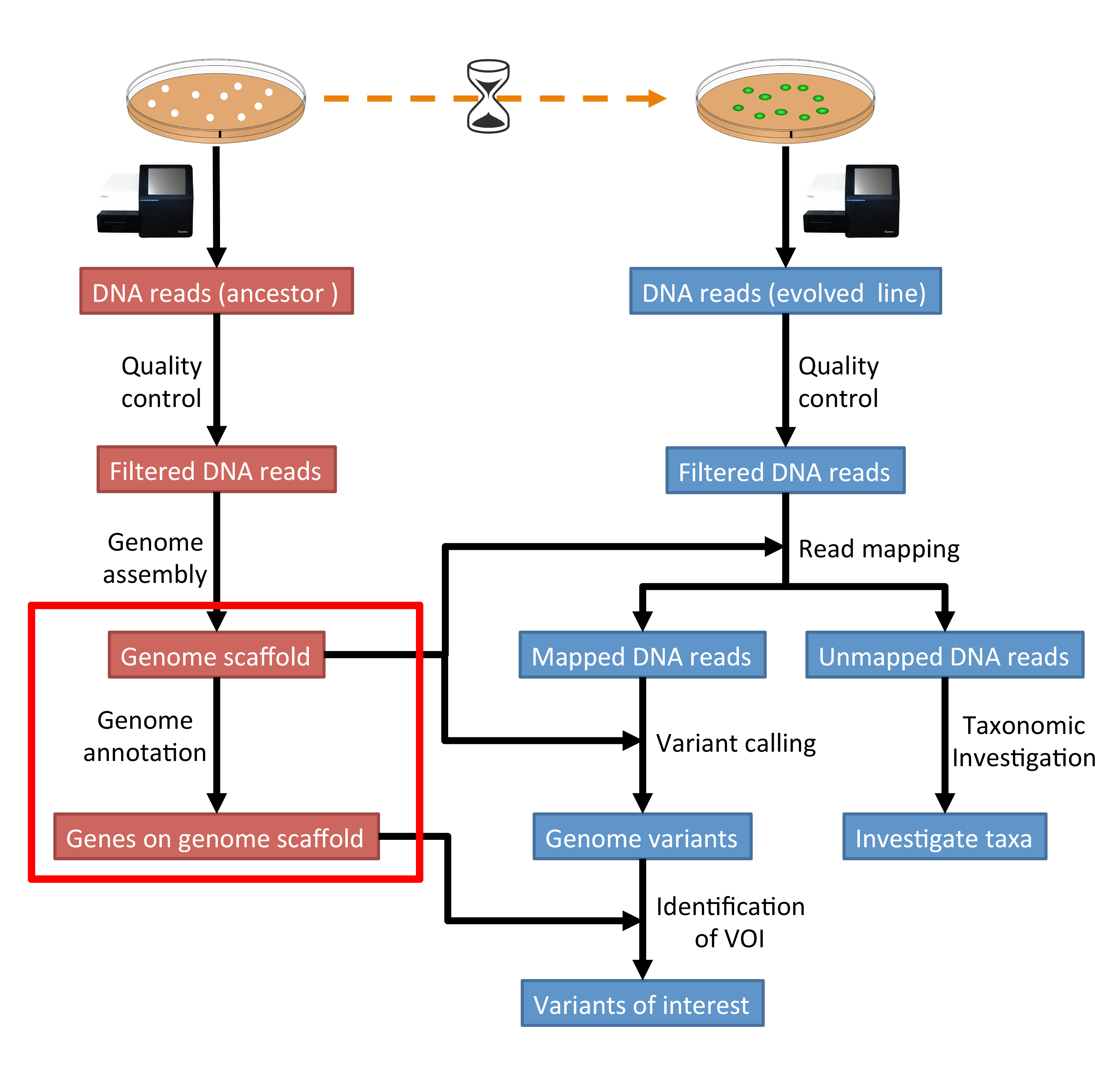
Fig. 8.1 The part of the workflow we will work on in this section marked in red.
8.3. Learning outcomes
After studying this section of the tutorial you should be able to:
Explain how annotation completeness is assessed using orthologues
Use bioinformatics tools to perform gene prediction
Use genome-viewing software to graphically explore genome annotations and NGS data overlays
8.4. Before we start
Lets see how our directory structure looks so far:
cd ~/analysis
ls -1F
assembly/
data/
kraken/
mappings/
trimmed/
trimmed-fastqc/
variants/
8.5. Installing the software
# activate the env
conda activate ngs

conda install busco
This will install both the Augustus [STANKE2005] and the BUSCO [SIMAO2015] software, which we will use (separately) for gene prediction and assessment of assembly completeness, respectively.
Make a directory for the annotation results:
mkdir annotation
cd annotation
We need to get the database that BUSCO will use to assess orthologue presence absence in our genome annotation. We will use wget for this:
wget http://busco.ezlab.org/datasets/saccharomycetales_odb9.tar.gz

# unpack the archive
tar -xzvf saccharomycetales_odb9.tar.gz
Note
Should the download fail, download manually from Downloads.
We also need to place the configuration file for this program in a location in which we have “write” privileges. Do this recursively for the entire config directory, placing it into your current annotation directory:
cp -r ~/miniconda3/envs/ngs/config/ ./
We next need to specify the path to this config file so that the program knows where to look now that we have changed the location (note that this is all one line below):
export AUGUSTUS_CONFIG_PATH="~/analysis/annotation/config/"n
We next check that we have actually changed the path correctly.
Entering this into the command should result in the file location being output on the next line of the command prompt.
echo $AUGUSTUS_CONFIG_PATH
8.6. Assessment of orthologue presence and absence
BUSCO will assess orthologue presence absence using blastn, a rapid method of finding close matches in large databases (we will discuss this in lecture). It uses blastn to make sure that it does not miss any part of any possible coding sequences. To run the program, we give it
A fasta format input file
A name for the output files
The name of the lineage database against which we are assessing orthologue presence absence (that we downloaded above)
An indication of the type of annotation we are doing (genomic, as opposed to transcriptomic or previously annotated protein files).
busco -i ../assembly/spades_final/scaffolds.fasta -o file_name_of_your_choice -l ./saccharomycetales_odb9 -m geno
Note
This should take about 90 minutes to run. So in the meantime do the next step.
8.7. Annotation
We will use Augustus to perform gene prediction. This program implements a hidden markov model (HMM) to infer where genes lie in the assembly you have made. To run the program you need to give it:
Information as to whether you would like the genes called on both strands (or just the forward or reverse strands)
A “model” organism on which it can base it’s HMM parameters on (in this case we will use S. cerevisiae)
The location of the assembly file
A name for the output file, which will be a .gff (general feature format) file.
We will also tell it to display a progress bar as it moves through the genome assembly.
augustus --progress=true --strand=both --species=saccharomyces_cerevisiae_S288C ../assembly/spades_final/scaffolds.fasta > your_new_fungus.gff
Note
Should the process of producing your annotation fail, you can download a annotation manually from Downloads. Remember to unzip the file.
8.8. Interactive viewing
We will use the software IGV to view the assembly, the gene predictions you have made, and the variants that you have called, all in one window.
8.9. Installing IGV
We will not install this software using conda. Instead, make a new directory in your home directory entitled “software”, and change into this directory. You will have to download the software from the Broad Institute:
mkdir software
cd software
wget http://data.broadinstitute.org/igv/projects/downloads/2.4/IGV_2.4.10.zip

# unzip the software:
unzip IGV_2.4.10.zip

# and change into that directory.
cd IGV_2.4.10.zip

# To run the interactive GUI, you will need to run the bash script in that directory:
bash igv.sh
Note
Should the download fail, download manually from Downloads.
This will open up a new window. Navigate to that window and open up your genome assembly:
Genome -> load Genome from File
Load your assembly, not your gff file.
Load the tracks:
File -> Load from file
Load your
vcffile from last weekLoad your
gfffile from this week.
At this point you should be able to zoom in and out to see regions in which there are SNPs or other types of variants. You can also see the predicted genes. If you zoom in far enough, you can see the sequence (DNA and protein).
If you have time and interest, you can right click on the sequence and copy it. Open a new browser window and go to the blastn homepage. There, you can blast your gene of interest (GOI) and see if blast can assign a function to it.
The end goal of this lab will be for you to select a variant that you feel is interesting (e.g. due to the gene it falls near or within), and hypothesize as to why that mutation might have increased in frequency in these evolving yeast populations.
8.10. Assessment of orthologue presence and absence (2)
Hopefully your BUSCO analysis will have finished by this time.
Navigate into the output directory you created.
There are many directories and files in there containing information on the orthologues that were found, but here we are only really interested in one: the summary statistics.
This is located in the short_summary*.txt file.
Look at this file.
It will note the total number of orthologues found, the number expected, and the number missing.
This gives an indication of your genome completeness.
Todo
Is it necessarily true that your assembly is incomplete if it is missing some orthologues? Why or why not?
References
- SIMAO2015
Simao FA, Waterhouse RM, Ioannidis P, Kriventseva EV and Zdobnov EM. BUSCO: assessing genome assembly and annotation completeness with single-copy orthologs. Bioinformatics, 2015, Oct 1;31(19):3210-2
- STANKE2005
Stanke M and Morgenstern B. AUGUSTUS: a web server for gene prediction in eukaryotes that allows user-defined constraints. Nucleic Acids Res, 2005, 33(Web Server issue): W465–W467.