5. Read mapping
5.1. Preface
In this section we will use our skill on the command-line interface to map our reads from the evolved line to our ancestral reference genome.
Note
You will encounter some To-do sections at times. Write the solutions and answers into a text-file.
5.2. Overview
The part of the workflow we will work on in this section can be viewed in Fig. 5.1.
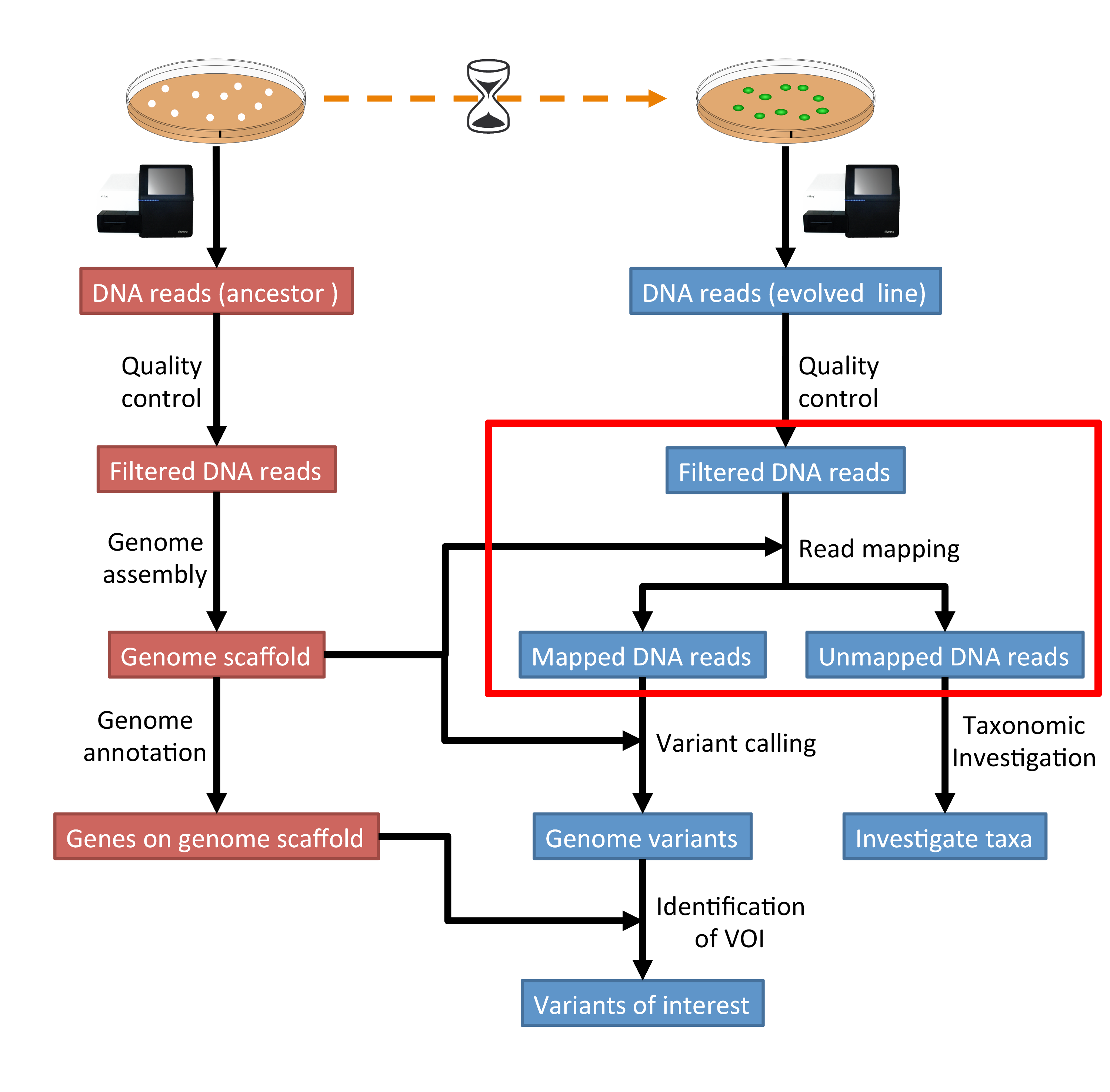
Fig. 5.1 The part of the workflow we will work on in this section marked in red.
5.3. Learning outcomes
After studying this section of the tutorial you should be able to:
Explain the process of sequence read mapping.
Use bioinformatics tools to map sequencing reads to a reference genome.
Filter mapped reads based on quality.
5.4. Before we start
Lets see how our directory structure looks so far:
cd ~/analysis
# create a mapping result directory
mkdir mappings
ls -1F
assembly/
data/
mappings/
(sampled/)
trimmed/
trimmed-fastqc/
Attention
If you sampled reads randomly for the assembly tutorial in the last section, please go and download first the assembly on the full data set. This can be found under Downloads. Unarchive and uncompress the files with tar -xvzf assembly.tar.gz.
5.5. Mapping sequence reads to a reference genome
We want to map the sequencing reads to the ancestral reference genome we created in the section Genome assembly. We are going to use the quality trimmed forward and backward DNA sequences of the evolved line and use a program called BWA to map the reads.
Todo
Discuss briefly why we are using the ancestral genome as a reference genome as opposed to a genome for the evolved line.
5.6. BWA
5.6.1. Overview
BWA is a short read aligner, that can take a reference genome and map single- or paired-end data to it [LI2009]. It requires an indexing step in which one supplies the reference genome and BWA will create an index that in the subsequent steps will be used for aligning the reads to the reference genome. The general command structure of the BWA tools we are going to use are shown below:
# bwa index help
bwa index

# indexing
bwa index path/to/reference-genome.fa

# bwa mem help
bwa mem

# single-end mapping, general command structure, adjust to your case
bwa mem path/to/reference-genome.fa path/to/reads.fq.gz > path/to/aln-se.sam

# paired-end mapping, general command structure, adjust to your case
bwa mem path/to/reference-genome.fa path/to/read1.fq.gz path/to/read2.fq.gz > path/to/aln-pe.sam
5.6.2. Creating a reference index for mapping
Todo
Create an BWA index for our reference genome assembly. Attention! Remember which file you need to submit to BWA.
Hint
Should you not get it right, try the commands in Code: BWA indexing.
5.6.3. Mapping reads in a paired-end manner
Now that we have created our index, it is time to map the filtered and trimmed sequencing reads of our evolved line to the reference genome.
Todo
Use the correct bwa mem command structure from above and map the reads of the evolved line to the reference genome.
Hint
Should you not get it right, try the commands in Code: BWA mapping.
5.7. Bowtie2 (alternative to BWA)
Attention
If the mapping did not succeed with BWA. We can use the aligner Bowtie2 explained in this section. If the mapping with BWA did work, you can jump this section. You can jump straight ahead to Section 5.8.
Install with:
conda install bowtie2
5.7.1. Overview
Bowtie2 is a short read aligner, that can take a reference genome and map single- or paired-end data to it [TRAPNELL2009]. It requires an indexing step in which one supplies the reference genome and Bowtie2 will create an index that in the subsequent steps will be used for aligning the reads to the reference genome. The general command structure of the Bowtie2 tools we are going to use are shown below:
# bowtie2 help
bowtie2-build

# indexing
bowtie2-build genome.fasta /path/to/index/prefix

# paired-end mapping
bowtie2 -X 1000 -x /path/to/index/prefix -1 read1.fq.gz -2 read2.fq.gz -S aln-pe.sam
-X: Adjust the maximum fragment size (length of paired-end alignments + insert size) to 1000bp. This might be useful if you do not know the exact insert size of your data. The Bowtie2 default is set to 500 which is often considered too short.
5.7.2. Creating a reference index for mapping
Todo
Create an Bowtie2 index for our reference genome assembly. Attention! Remember which file you need to submit to Bowtie2.
Hint
Should you not get it right, try the commands in Code: Bowtie2 indexing.
5.7.3. Mapping reads in a paired-end manner
Now that we have created our index, it is time to map the filtered and trimmed sequencing reads of our evolved line to the reference genome.
Todo
Use the correct bowtie2 command structure from above and map the reads of the evolved line to the reference genome.
Hint
Should you not get it right, try the commands in Code: Bowtie2 mapping.
Note
Bowtie2 does give very cryptic error messages without telling much why it did not want to run. The most likely reason is that you specified the paths to the files and result file wrongly. Check this first. Use tab completion a lot!
5.8. The sam mapping file-format
Bowtie2 and BWA will produce a mapping file in sam-format. Have a look into the sam-file that was created by either program. A quick overview of the sam-format can be found here and even more information can be found here. Briefly, first there are a lot of header lines. Then, for each read, that mapped to the reference, there is one line.
The columns of such a line in the mapping file are described in Table 5.1.
Col |
Field |
Description |
|---|---|---|
1 |
QNAME |
Query (pair) NAME |
2 |
FLAG |
bitwise FLAG |
3 |
RNAME |
Reference sequence NAME |
4 |
POS |
1-based leftmost POSition/coordinate of clipped sequence |
5 |
MAPQ |
MAPping Quality (Phred-scaled) |
6 |
CIAGR |
extended CIGAR string |
7 |
MRNM |
Mate Reference sequence NaMe (‘=’ if same as RNAME) |
8 |
MPOS |
1-based Mate POSition |
9 |
ISIZE |
Inferred insert SIZE |
10 |
SEQ |
query SEQuence on the same strand as the reference |
11 |
QUAL |
query QUALity (ASCII-33 gives the Phred base quality) |
12 |
OPT |
variable OPTional fields in the format TAG:VTYPE:VALUE |
One line of a mapped read can be seen here:
M02810:197:000000000-AV55U:1:1101:10000:11540 83 NODE_1_length_1419525_cov_15.3898 607378 60 151M = 607100 -429 TATGGTATCACTTATGGTATCACTTATGGCTATCACTAATGGCTATCACTTATGGTATCACTTATGACTATCAGACGTTATTACTATCAGACGATAACTATCAGACTTTATTACTATCACTTTCATATTACCCACTATCATCCCTTCTTTA FHGHHHHHGGGHHHHHHHHHHHHHHHHHHGHHHHHHHHHHHGHHHHHGHHHHHHHHGDHHHHHHHHGHHHHGHHHGHHHHHHFHHHHGHHHHIHHHHHHHHHHHHHHHHHHHGHHHHHGHGHHHHHHHHEGGGGGGGGGFBCFFFFCCCCC NM:i:0 MD:Z:151 AS:i:151 XS:i:0
It basically defines, the read and the position in the reference genome where the read mapped and a quality of the map.
5.9. Mapping post-processing
5.9.1. Fix mates and compress
Because aligners can sometimes leave unusual SAM flag information on SAM records, it is helpful when working with many tools to first clean up read pairing information and flags with SAMtools.
We are going to produce also compressed bam output for efficient storing of and access to the mapped reads.
Note, samtools fixmate expects name-sorted input files, which we can achieve with samtools sort -n.
samtools sort -n -O sam mappings/evolved-6.sam | samtools fixmate -m -O bam - mappings/evolved-6.fixmate.bam
-m: Add ms (mate score) tags. These are used by markdup (below) to select the best reads to keep.-O bam: specifies that we want compressed bam output from fixmate
Attention
The step of sam to bam-file conversion might take a few minutes to finish, depending on how big your mapping file is.
We will be using the SAM flag information later below to extract specific alignments.
Hint
A very useful tools to explain flags can be found here.
Once we have bam-file, we can also delete the original sam-file as it requires too much space.
rm mappings/evolved-6.sam
5.9.2. Sorting
We are going to use SAMtools again to sort the bam-file into coordinate order:
# convert to bam file and sort
samtools sort -O bam -o mappings/evolved-6.sorted.bam mappings/evolved-6.fixmate.bam
-o: specifies the name of the output file.-O bam: specifies that the output will be bam-format
5.9.3. Remove duplicates
In this step we remove duplicate reads. The main purpose of removing duplicates is to mitigate the effects of PCR amplification bias introduced during library construction. It should be noted that this step is not always recommended. It depends on the research question. In SNP calling it is a good idea to remove duplicates, as the statistics used in the tools that call SNPs sub-sequently expect this (most tools anyways). However, for other research questions that use mapping, you might not want to remove duplicates, e.g. RNA-seq.
samtools markdup -r -S mappings/evolved-6.sorted.bam mappings/evolved-6.sorted.dedup.bam
Todo
Figure out what “PCR amplification bias” means.
Note
Should you be unable to do the post-processing steps, you can download the mapped data from Downloads.
5.10. Mapping statistics
5.10.1. Stats with SAMtools
Lets get an mapping overview:
samtools flagstat mappings/evolved-6.sorted.dedup.bam
Todo
Look at the mapping statistics and understand their meaning. Discuss your results. Explain why we may find mapped reads that have their mate mapped to a different chromosome/contig? Can they be used for something?
For the sorted bam-file we can get read depth for at all positions of the reference genome, e.g. how many reads are overlapping the genomic position.
samtools depth mappings/evolved-6.sorted.dedup.bam | gzip > mappings/evolved-6.depth.txt.gz
Todo
Extract the depth values for contig 20 and load the data into R, calculate some statistics of our scaffold.
zcat mappings/evolved-6.depth.txt.gz | egrep '^NODE_20_' | gzip > mappings/NODE_20.depth.txt.gz
Now we quickly use some R to make a coverage plot for contig NODE20.
Open a R shell by typing R on the command-line of the shell.
x <- read.table('mappings/NODE_20.depth.txt.gz', sep='\t', header=FALSE,  strip.white=TRUE)

# Look at the beginning of x
head(x)

# calculate average depth
mean(x[,3])
# std dev
sqrt(var(x[,3]))

# mark areas that have a coverage below 20 in red
plot(x[,2], x[,3], col = ifelse(x[,3] < 20,'red','black'), pch=19, xlab='postion', ylab='coverage')

# to save a plot
png('mappings/covNODE20.png', width = 1200, height = 500)
plot(x[,2], x[,3], col = ifelse(x[,3] < 20,'red','black'), pch=19, xlab='postion', ylab='coverage')
dev.off()
The result plot will be looking similar to the one in Fig. 5.2
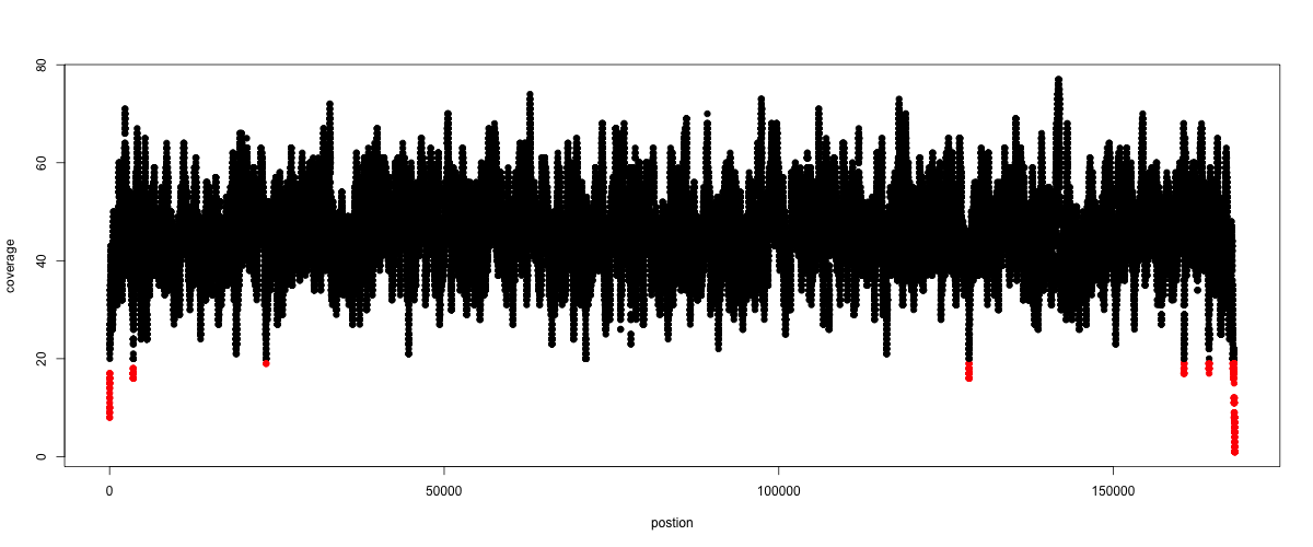
Fig. 5.2 A example coverage plot for a contig with highlighted in red regions with a coverage below 20 reads.
Todo
Look at the created plot. Explain why it makes sense that you find relatively bad coverage at the beginning and the end of the contig.
5.10.2. Stats with QualiMap
For a more in depth analysis of the mappings, one can use QualiMap [OKO2015].
QualiMap examines sequencing alignment data in SAM/BAM files according to the features of the mapped reads and provides an overall view of the data that helps to the detect biases in the sequencing and/or mapping of the data and eases decision-making for further analysis.
Installation:
conda install qualimap
Run QualiMap with:
qualimap bamqc -bam mappings/evolved-6.sorted.dedup.bam
This will create a report in the mapping folder. See this webpage to get help on the sections in the report.
Todo
Install QualiMap and investigate the mapping of the evolved sample. Write down your observations.
5.11. Sub-selecting reads
It is important to remember that the mapping commands we used above, without additional parameters to sub-select specific alignments (e.g. for Bowtie2 there are options like --no-mixed, which suppresses unpaired alignments for paired reads or --no-discordant, which suppresses discordant alignments for paired reads, etc.), are going to output all reads, including unmapped reads, multi-mapping reads, unpaired reads, discordant read pairs, etc. in one file.
We can sub-select from the output reads we want to analyse further using SAMtools.
Todo
Explain what concordant and discordant read pairs are? Look at the Bowtie2 manual.
5.11.1. Concordant reads
We can select read-pair that have been mapped in a correct manner (same chromosome/contig, correct orientation to each other, distance between reads is not stupid).
samtools view -h -b -f 3 mappings/evolved-6.sorted.dedup.bam > mappings/evolved-6.sorted.dedup.concordant.bam
-h: Include the sam header-b: Output will be bam-format-f 3: Only extract correctly paired reads.-fextracts alignments with the specified SAM flag set.
Todo
Our final aim is to identify variants. For a particular class of variants, it is not the best idea to only focus on concordant reads. Why is that?
5.11.2. Quality-based sub-selection
In this section we want to sub-select reads based on the quality of the mapping. It seems a reasonable idea to only keep good mapping reads. As the SAM-format contains at column 5 the \(MAPQ\) value, which we established earlier is the “MAPping Quality” in Phred-scaled, this seems easily achieved. The formula to calculate the \(MAPQ\) value is: \(MAPQ=-10*log10(p)\), where \(p\) is the probability that the read is mapped wrongly. However, there is a problem! While the MAPQ information would be very helpful indeed, the way that various tools implement this value differs. A good overview can be found here. Bottom-line is that we need to be aware that different tools use this value in different ways and the it is good to know the information that is encoded in the value. Once you dig deeper into the mechanics of the \(MAPQ\) implementation it becomes clear that this is not an easy topic. If you want to know more about the \(MAPQ\) topic, please follow the link above.
For the sake of going forward, we will sub-select reads with at least medium quality as defined by Bowtie2:
samtools view -h -b -q 20 mappings/evolved-6.sorted.dedup.bam > mappings/evolved-6.sorted.dedup.q20.bam
-h: Include the sam header-q 20: Only extract reads with mapping quality >= 20
Hint
I will repeat here a recommendation given at the source link above, as it is a good one: If you unsure what \(MAPQ\) scoring scheme is being used in your own data then you can plot out the \(MAPQ\) distribution in a BAM file using programs like the mentioned QualiMap or similar programs. This will at least show you the range and frequency with which different \(MAPQ\) values appear and may help identify a suitable threshold you may want to use.
5.11.3. Unmapped reads
We could decide to use Kraken2 like in section Taxonomic investigation to classify all unmapped sequence reads and identify the species they are coming from and test for contamination.
Lets see how we can get the unmapped portion of the reads from the bam-file:
samtools view -b -f 4 mappings/evolved-6.sorted.dedup.bam > mappings/evolved-6.sorted.unmapped.bam

# count them
samtools view -c mappings/evolved-6.sorted.unmapped.bam
-b: indicates that the output is BAM.-f INT: only include reads with this SAM flag set. You can also use the commandsamtools flagsto get an overview of the flags.-c: count the reads
Lets extract the fastq sequence of the unmapped reads for read1 and read2.
bamToFastq -i mappings/evolved-6.sorted.unmapped.bam -fq mappings/evolved-6.sorted.unmapped.R1.fastq -fq2 mappings/evolved-6.sorted.unmapped.R2.fastq
References
- TRAPNELL2009
Trapnell C, Salzberg SL. How to map billions of short reads onto genomes. Nat Biotechnol. (2009) 27(5):455-7. doi: 10.1038/nbt0509-455.
- LI2009
Li H, Durbin R. (2009). Fast and accurate short read alignment with Burrows-Wheeler transform. Bioinformatics. 25 (14): 1754–1760.
- OKO2015
Okonechnikov K, Conesa A, García-Alcalde F. Qualimap 2: advanced multi-sample quality control for high-throughput sequencing data. Bioinformatics (2015), 32, 2:292–294.